Willow Software User Manual

System Overview

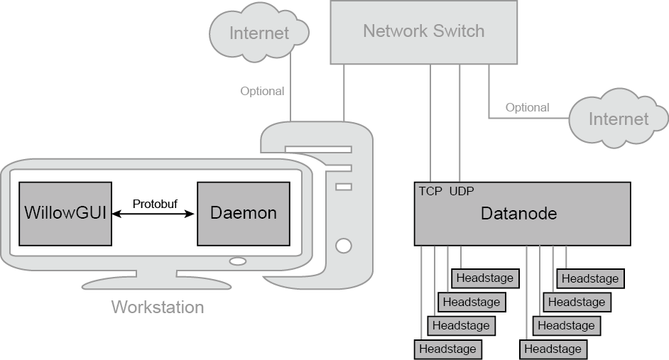
The Willow system is comprised of both hardware and software components. On the hardware side, there is the Datanode, which is the main data acquisition and storage computer. The Datanode collects data from the headstages, which are modular amplifier and digitizer boards. Each headstage acquires from 128 channels, and each Datanode can collect from as many as 8 headstages. The Datanode receives commands from the workstation - a computer running Linux. The Datanode and the workstation communicate over a high-speed Ethernet connection.

The workstation itself runs a multi-layered software stack. The Daemon handles the low-level communication with the Datanode, data collection, routing, and I/O. The daemon exposes a control interface based on Google’s Protocol Buffers (protobuf). The WillowGUI software wraps this control interface in some higher-level functions that allow the user to record, stream, an analyze data with the convenience of a graphical user interface.

Note

As of Willow 2.0, Linux is the only supported operating system.

Daemon

Install

Skip to the Network Configuration section if the Willow system is pre-configured from LeafLabs or the workstation has already been setup for Willow.

Note

This guide assumes an apt-based Linux distribution (Debian, Ubuntu, Mint, etc.) with standard packages like git and Python 2.7 installed. WillowGUI has only been tested on Ubuntu 16.04.

First, download the daemon source code:

$ git clone https://github.com/leaflabs/willow-daemon.git
$ cd willow-daemon

Open willow-daemon/README.txt, and install all mandatory dependencies described therein. Then, compile the daemon using scons:

$ cd willow-daemon
$ scons EXTRA_FLAGS='-O2'

The resulting executable should be in build/.

Network Configuration

A pre-configured workstation from LeafLabs has two NICs - one built-in to the motherboard (labelled Internet) and a second as a PCI card (labelled Willow) - to allow internet access while communicating with the WiIlow datanode. Each NIC is configured for one purpose or the other but not both. Thus, it is important to establish correct connectivity by following the labels.

In case the labels are missing or illegible, correct connectivity can still be determined. To begin, in the case of reversed connectivity, WillowGUI will display no connectivity to DataNode (even though the datanode can be pinged at 192.168.1.2) and no IP address will be issued by DHCP to NIC intended for internet (as seen by running ipconfig at a command prompt). To restore proper function, swap the ethernet cables connected to the workstation. WillowGUI will display no connectivity to Datanode (see Figure 7.) even though the datanode can be pinged at 192.168.1.2, and no IP address will be issued by DHCP to NIC intended for internet (as seen by running ipconfig at a command prompt). To restore proper function, swap the ethernet cables connected to the workstation.

To support high data rate network traffic, it is important configure the size in bytes of network packets. If you’re using a pre-configured Willow workstation, this happens automatically upon startup. In the case of a non-pre-configured workstation, a utility script is included with the Daemon in willow-daemon/util:

$ cd leafysd/util
$ ./expand_eth_buffers.sh <interface>

where <interface> is the name of your network interface (default is eth0).

Note

This script requires sudo privileges. See Login to the Workstation.

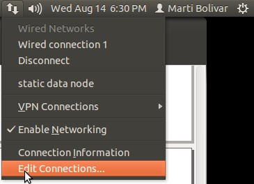
On a pre-configured Willow workstation, the network configuration is already set. Alternatively, to manually set up the network interface for Willow, start Network Connection Editor, either from a terminal:

$ nm-connection editor

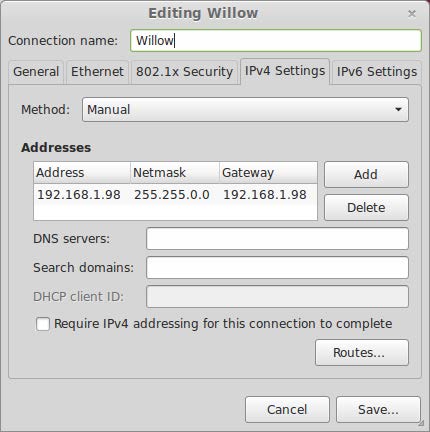
or (on Ubuntu) by clicking “Edit Connections” in the Network Connections dropdown in the menu bar. Add a new Ethernet connection, and call it “Willow”. In the IPv4 Settings tab, set the “Method” to “Manual”, then add a new address with Address=192.168.1.98, Netmask=255.255.0.0, and Gateway=192.168.1.98. Click “Save”, and close the Connection Editor.

Note

The Willow local area network domain is hard-coded in the FPGA on the Datanode to be 192.168.1.XXX. However, this same network domain is not uncommon for LANs. Thus, there is the potential for IP address conflict.

WillowGUI

Introduction

This is the user guide for the Willow GUI software: a desktop application for interacting with Willow, a 1024-channel electrophysiology system developed by LeafLabs in collaboration with MIT’s Synthetic Neurobiology Group (SNG). This document, contains information for end-users. Developers should check out the developer’s guide.

System Overview

The Willow board communicates over TCP and UDP connections with a workstation computer running a daemon server called willow-daemon. All interactions with the hardware go through the daemon, which exposes an interface based on Google’s Protocol Buffers (protobuf). The daemon repository includes command-line utilities for sending and receiving protobuf messages to and from the daemon. The GUI was designed to replace the command-line workflow with a more accessible and streamlined graphical approach.

This setup guide assumes you have already installed the daemon and configured your network; if not, refer to the Willow 2.0 User Guide for instructions on how to do this.

Install

To access the GUI repository, clone it from GitHub:

$ git clone https://github.com/leaflabs/willowgui.git

This will create in the current directory a local copy of the repository in a folder named willowgui. Before running the GUI, you’ll need to install these mandatory dependencies:

$ sudo apt-get install python-numpy python-matplotlib python-qt4 python-tk \
      python-git python-scipy python-pyqtgraph python-h5py hdfview

GUI Startup

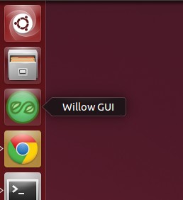
On a pre-configured Willow workstation, you can start WillowGUI by clicking the WillowGUI icon on the Unity Launcher side panel.

Alternatively, you can start WillowGUI from the top-level folder of the local repository (e.g. willowgui) with

$ src/main.py

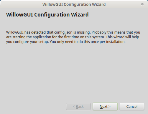
The first time you run the GUI, a Configuration Wizard will appear. Follow the instructions and click Finish.

If the setup was successful, the WillowGUI control panel will appear on the screen.

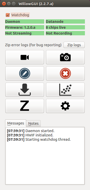
Usage

The Willow Control Panel (pictured above) consists of the status bar, the button panel, and the message log. The daemon is automatically started in the background, with stderr and stdout redirected to log/eFile and log/oFile, respectively. The message log should display a line indicating that the daemon was started successfully.

Status Bar

The status bar is an array of labels at the top of the main window, which indicates the status of the daemon and the hardware. The status bar is updated by a watchdog process which pings the Datanode once every second, and evaluates the response to determine daemon status, Datanode status, firmware version, hardware (i.e. neural chip) status, streaming state, and recording state. The general color code for the labels is: green for “good/normal state”, orange for “bad state, something is wrong”, and gray for “unknown state”. For example, if the Datanode is unresponsive, its label will turn orange and the labels below it will turn gray to indicate an unknown state. Similarly, if the daemon is unresponsive, its label will turn orange and all labels below it will turn gray. These conditions are shown below.

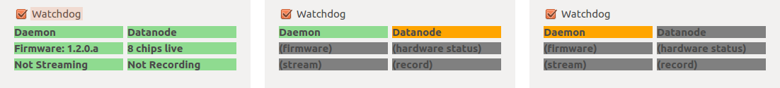
Figure 7. Status bar in three states: Daemon up and connected to Datanode, showing firmware version, number of chips alive, and streaming/recording states (left); Daemon up but Datanode unresponsive (center); Daemon down or unreachable, hardware state unknown (right).

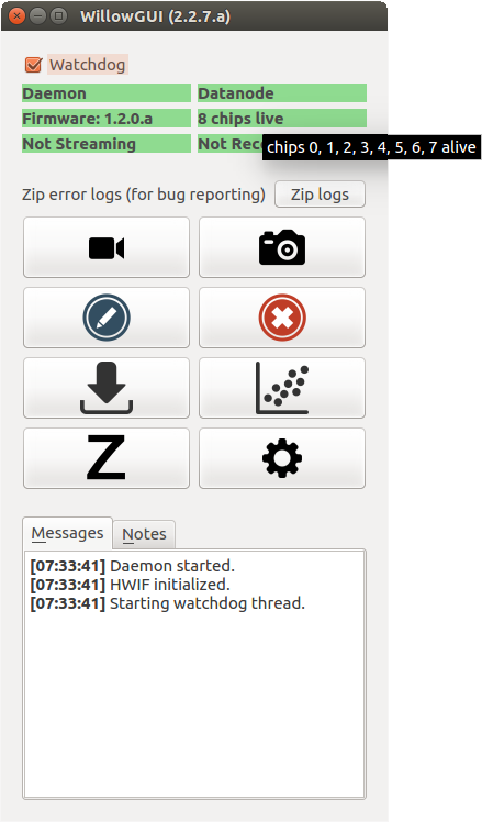
The firmware label, when green, will show the firmware version as a 32-bit hexadecimal number. The hardware status label beside it indicates the number of active neural chips that were found. Hovering over the label will display the id’s (0-based) of the active chips. For example, MISO/MOSI1 corresponds to chips 0,1,2,3; MISO/MOSI2 corresponds to active chips 4,5,6,7; etc. Note chips are numbered from left to right on the headstage as viewed in Figure 3..

Note

Hardware-related bug reports can be sent to info@leaflabs.com, and should include both the firmware version and the error state bitmask as context.

The Stream label indicates the streaming state of the Datanode: green for idle, and blue for streaming. Similarly, the Record label beside it is green for idle, but turns red while recording and additionally indicates the current disk usage as a percentage in real time. These states — streaming and recording — are determined from the hardware registers on the Datanode, and are therefore robust to daemon and/or GUI crashes.

The Watchdog process can be disabled by un-checking the Watchdog box at the top of the status bar. This should rarely be necessary, but may free up some bandwidth during streaming or transfer operations on slow workstations. The status bar will no longer be updated while the Watchdog is disabled.

Message Log

At the bottom of the main window is the message log, which displays and logs messages from the GUI. Examples of messages include success/failure reports from requested actions, status updates from background threads, and general errors. Each message is prepended with a timestamp of the form HH:mm:ss. The message log can be cleared, or saved to a log file using the buttons at the top-right. Message logs are saved to the log/ subdirectory by default, but can be saved anywhere by navigating the presented file dialog.

The message log is intended to serve as a supplement to the experimentalist’s lab notebook, logging the actions taken — and their results — to help contextualize the data for future analysis.

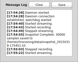
Figure 8. The message log, showing a list of actions taken, with timestamps.

Button Panel

At the center of the main GUI window is the button panel, containing 8 buttons with symbolic icons. These buttons are your starting point for all the capabilities offered by the GUI. Mousing over a button will display a tooltip which describes its action.

Streaming

UPDATE

Snapshots

UPDATE

Recording

Recording is the acquisition of data directly to the SATA disk. It is the only acquisition mode that is guaranteed to be robust, and is intended for scientific experiments. To start a recording, click the Start Recording button in the Button Panel. The corresponding label in the status bar will turn from green to red, and the label will begin displaying the disk usage. Accurate reporting of disk usage is depending on the Datanode Storage Capacity parameter in your settings. To stop recording, click the Stop Recording button.

Warning

Every time you click Start, the system will start recording from the beginning of the disk, over-writing any previous experiments you may have recorded. In this sense, the disk acts as a temporary (non-volatile) buffer for experimental data. If you’ve just recorded an experiment and want to preserve the data, it is recommended that you transfer the data over to your workstation immediately after stopping recording. If storage space is an issue on your workstation, an alternative is to remove the SATA disk and label it, thus repurposing the disk buffer as an archival system.

Note

Filling the SSD with data to 100% capacity (as defined by Datanode Storage Capacity in Settings) is allowed. In this case, WillowGUI will briefly indicate that 100% capacity was achieved (REF FIGURE), will report the final sample index (THAT WAS LAST WRITTEN?), and will stop the recording. Importantly, the criterion for stopping the recording is that Datanode Storage Capacity was reached, not necessarily that the SSD actually is full. Thus, normal operation of WillowGUI is expected when Datanode Storage Capacity is less than or equal to the actual capacity of the SSD. For details on what to expect when SSD capacity is less than Datanode Storage Capacity, see Troubleshooting.

Transferring Experiments

ADD CONTENT.

Experiments cannot be transferred while recording. The recording must be stopped before the experimental data can be transferred.

Plotting Data

ADD CONTENT.

Impedance Testing

The Intan headstages offer impedance testing functionality which can be accessed from the GUI. Click the Run Impedance Test button on the button panel — this will present a dialog where you can choose to measure the impedance of a single channel, or of all channels in sequence. If you choose Single Channel, the process will take about 10 seconds, and the result will be posted on the message log. If you choose All Channels, the loop will run for about 3 minutes, and the result will be saved in a time-stamped .npy file, also reported in the message log. In All Channels mode, you also have the option to Plot When Finished, which will bring up a plot window showing the impedance results across all channels (see Figure 9.). All impedance measurements are taken at f = 1/kHz.

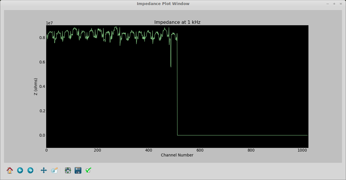
Figure 9. UPDATE FIGURE Impedance results from a measurement taken with 4 of 8 headstages bare headstages connected. As expected, channels 0-511 show an approximate, 32-channel periodicity from the PCB traces, and channels 512-1023 are dead.

Note

Impedance cannot be measured while recording. The Intan chips used in our headstages simply do not allow this.

Settings

The GUI preferences can be viewed and modified by clicking the Configure Settings button on the button panel. This will present a key-value dialog (see figure below) for the various configuration parameters. These values are stored in src/config.json, and persist across restarts.

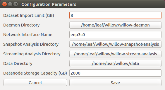
Figure 10. Settings window, showing default configuration parameters.

Troubleshooting

dffdsfgds

Working with Different Probe Geometries

dffdsfgds

Plugin Analysis Scripts

Describe Plugin Architecture of WillowGUI. Mention existing Plugin scripts.

Install

To access the snapshot analysis repository, clone it from GitHub:

$ git clone https://github.com/leaflabs/willow-snapshot-analysis.git

Likewise, to access the stream analysis repository, clone it from GitHub:

$ git clone https://github.com/leaflabs/willow-stream-analysis.git

ADD NOTE ABOUT DEPENDENCIES, IF ANY.

For Each Script, Walk through Functionality

dffdsfgds

Adding User Scripts

To add an analysis program to WillowGUI, create a new folder in the top level and put inside of it an executable named ‘main’. This executable can be anything - a MATLAB script, a Python GUI, a compiled program, etc. The only requirement is that is take as its first command-line argument the absolute filename of the snapshot it is to analyze.

To make this work with WillowGUI, set the Snapshot Analysis Directory parameter in the Config Wizard, or else in the Settings menu during runtime. Then, any subdirectory containing a ‘main’ executable will appear as an option for custom analysis in the Snapshot Dialog. WillowGUI will launch the executable as a subprocess, with its working directory set to that of the executable - so metadata (e.g. probe mappings) or library files can be kept in the same folder alongside the exectuable. stdout and stderr will be piped to ‘oFile’ and ‘eFile’ in the working directory, so avoid using these filenames for metadata, as they will get overwritten upon execution.

Place code or data that you’d like to re-use across different analysis programs in the lib/ directory. Then programs can access this code or data using relative pathnames, e.g. in Python:

sys.path.append('../lib/py')

Stay D.R.Y.; Don’t Repeat Yourself!

Working with Different Probe Geometries

dffdsfgds

Working with Data

The data on the SSDs is stored in raw form without a filesystem. This design choice simplifies the programming of the FPGA, but obviously is inconvenient and may change in future versions of Willow.

To read data off the SSD and into a file on a PC, the user has two options...

Retrieve Data from SSD Using WillowGUI

Immediately after an experiment ends (and before the Willow Datanode has been powered down!), data can be pulled from the SSD to the laptop (or whatever computer is controlling the Willow) using the WillowGUI.

1. From WillowGUI with Datanode connected, click Transfer (down-pointed arrow)
2. Under Experiment click Subset and select the time window, in seconds from start of recording

Note

After the Willow Datanode has been power cycled, the WillowGUI cannot be used retrieve data from an SSD. WHY NOT?!

Retrieve Data from SSD Using SATA-to-USB cable

Data can be pulled from SSDs at any time using the sata2hdf5 program that comes installed with the Daemon software. If not already done, first Install the daemon software. Then, using a SATA-to-USB adapter (one is included with every Willow system) attach to the PC one SSD, by first powering down the Willow Datanode and ejecting the SSD.

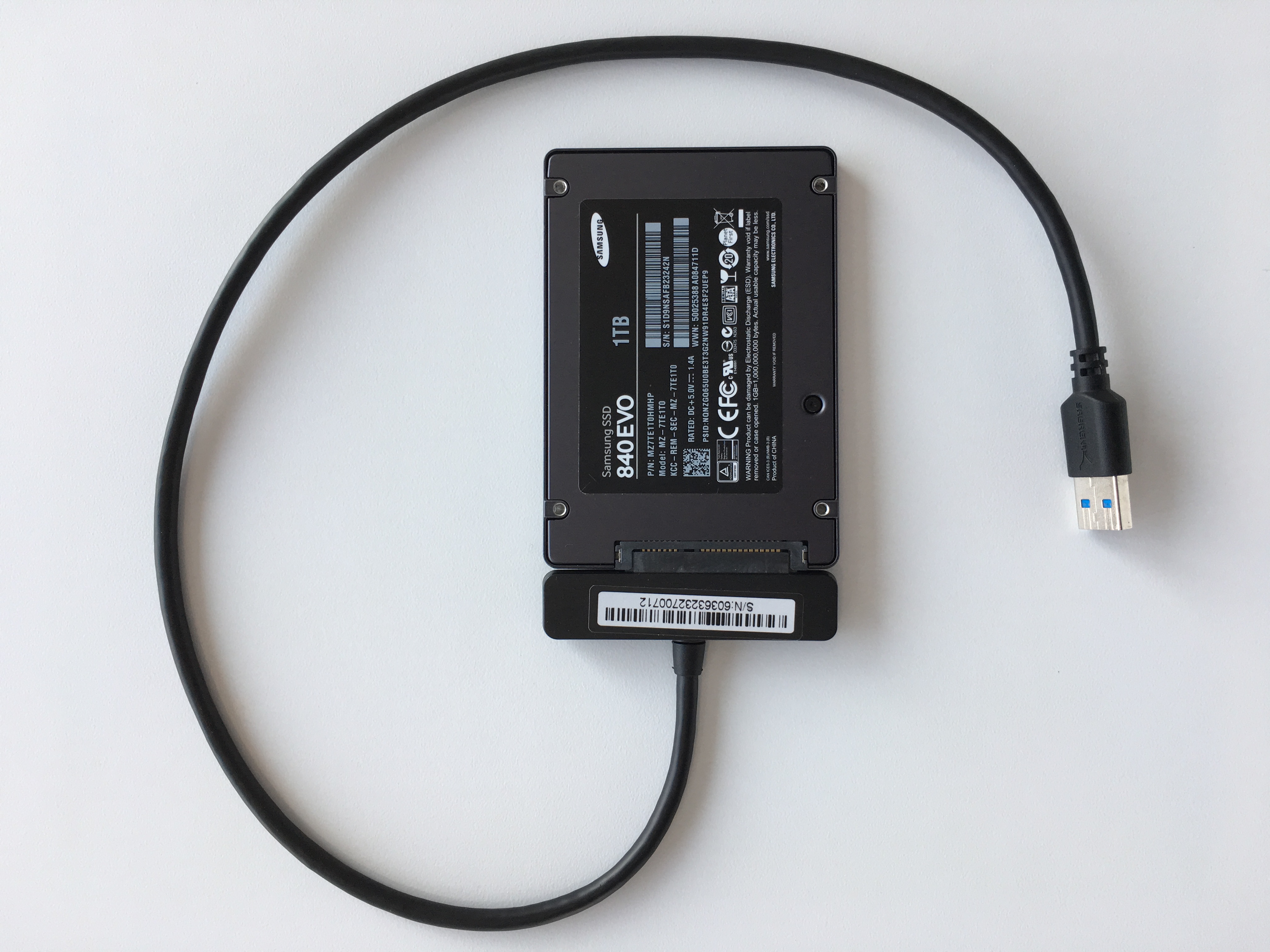
Figure 11. SATA-to-USB adapter with SSD attached.

Note

To ensure that the PC operating system quickly registers the SSD, connect the SSD to adapter first, then connect adapter to USB connector on PC.

Then,

1. Determine the device name assigned to USB-to-SATA adapter by running ls /dev/sd*` before and after attaching the adapter. The new device name is the desired one.
2. Determine the start time of data (recording on SSD), i.e. the UNIX time on the laptop when recording started.

Example:

$ sudo ~/src/willow-daemon/build/sata2hdf5 -c 30000 -o 0 /dev/sdd test.h5
Starting cookie: 0x57000886
Starting board id: 0x3746f441
Copied 30000...
Copied 30000 board samples.

0x57000886 = 1459619974 seconds since epoch = 2016-04-02 13:59:34+00:00 EST.

3. From snapshots (which have time embedded in filename), calculate the sample offset (which determines where in SSD to start extracting data). So, for data at 15:00 EST: sample offset = 15:00-14:00 = 60 minutes = 3600 sec = 3600*30e3 samples = 108000000.
4. Decide how many samples we want, e.g. 1 min = 60 sec*30e3 samples/sec = 1800000.
5. Finally, run sata2hdf5:

$ sudo ~/src/willow-daemon/build/sata2hdf5 -c 1800000 -o 108000000 /dev/sdd data_offset_1hr_length_1min.h5

Note

At this time obtaining a subset of the channels (e.g. 64 out of 1024) is not possible unfortunately, neither through WillowGUI or from sata2hdf5.

Finding a Snapshot in a Continous Recording

The situation may arise that a snapshot taken during an experiment contains particularly interesting data, and we wish to find that snapshot in a large continuous recording. To do so, see section Retrieve Data from SSD Using SATA-to-USB cable.

HDF5 version dependency

WillowGUI compiles without difficulty in Ubuntu 16.04 which include libhdf5 packages at version 1.8.16. Note that older versions of libhdf5 (e.g. version 1.8.11 as ships in Ubuntu 14.04) cause a compilation failure for WillowGUI (unless the signature for H5D_scatter_func_t in H5Dpublic.h is modifies with the addition of a const qualifier to the first argument).

Furthermore, Ubuntu 17.04 ships with version 1.10.0 of libhdf5. This is a major release jump, and this page: https://support.hdfgroup.org/HDF5/ warns that although HDF5-1.10 will read files created with earlier major releases, older releases such as HDF5-1.8 might not be able to read files created with HDF5-1.10. This could potentially cause headaches in the future, if e.g. a customer were to run sata2hdf5 on a system running Ubuntu 17.04, and then process the resulting file on a system running an older distro.

Opening HDF5 Files

The latest version of Ubuntu (16.04.2), which comes installed on any pre-configured workstation with the Willow system, includes HDFView for inspecting HDF5 files. Simply double-click on an HDF5 file to open the file and inspect its contents including all datasets and their attributes.

In addition, the WillowGUI can be used to interactively view HDF5 Snapshots.

HDF5 files in MATLAB

To open a snapshot HDF5 file in MATLAB, plot_snapshot.m is a script that accepts as input a filename and channels to plot. For example, to plot channel 128 from snapshot_20160402-161433_planetEarth.h5

plot_snapshot('snapshot_20160402-161433_planetEarth.h5',[128])

Generates as output

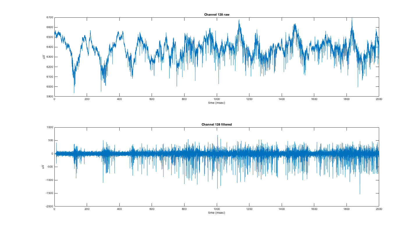
Figure 12. Plots of raw (top) and high-pass filtered (bottom) data for channel 128 in plot_snapshot(‘snapshot_20160402-161433_planetEarth.h5.

To open an impedance file, for example, impedance_20160402-130530.h5, in MATLAB run:

>> impedance = h5read(‘impedance_20160402-130530.h5’,'/impedanceMeasurements');
>> size(impedance)
ans =
      1024           1

Warning

In MATLAB, indexing of arrays is 1-based. In other words, the first element of any array (or along any dimension of a multi-dimensional array) is assigned an index of 1 and the last of N elements has an index of N. In contrast, the numbering and indexing of channels and chips in the Willow software suite is 0-based. This distinction is important when seeking to establish a correspondence between channels in Willow and other software packages such as MATLAB. Specifically, channel j in Willow is channel j+1 in MATLAB.

Snapshots with Aspen WDX

To interactively explore 1024 channel data sets, Aspen WDX utilizes a client-server interface to enable researchers to explore large TB-scale data sets using a thin client interface.

Channel Maps

To preserve the geometrical arrangement of recording sites on the probe when plotting neural data, a channel map is needed that describes which shank, row and column each channel occupies. Channel maps can be found in the willow-snapshot-analysis repository. For a more detailed treatment of channel maps see the probe-channel-maps repository in gitlab (MOVE OUT OF GITLAB). The nomenclature used in these channel maps is defined in this schematic (PDF):

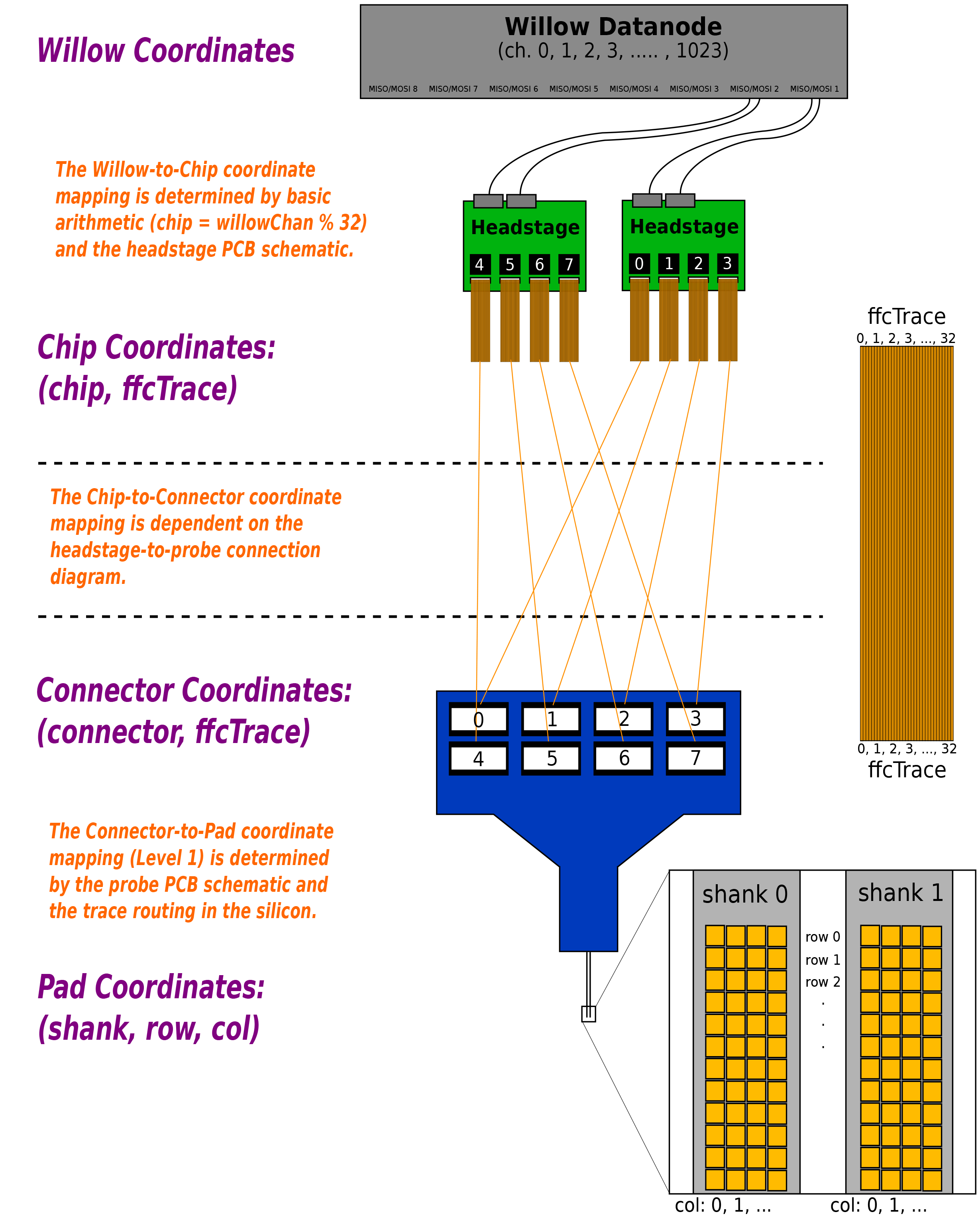
Figure 13. Nomenclature used to define channel maps.

Pre-configured Workstation

On a pre-configured workstation from LeafLabs, all willow-related software (the Willow Suite) is installed in ~/willow.

By default, WillowGUI saves data in ~/willow/data. Data can be saved to a different directory by configuring the Settings.

Documentation is contained in ~/willow/willow-docs.

All other subfolders of the ~/willow folder contain one component of the Willow software suite. Software components include willow-gui, willow-daemon, willow-docs, willow-snapshot-analysis, and willow-stream-analysis. Each component is a clone of a github repository.

To update any software component, cd into the subfolder of component, and run:

git pull origin master

If git responds that there were merge conflicts, it means that changes have been made to source code. In that case, you must resolve the conflicts before proceeding.

Frequently Asked Questions

Is there a way to update all Willow-related git repos at once?

Currently, no. But it would not be hard to write a bash script to do so, assuming that there were no changes made to local copy of the source code and no merge conflicts to resolve.